Time of Travel Charts for Low, Medium, and High Flows
on the Mississippi River above Minneapolis, Minnesota.
Table of Contents
Abstract
Travel times for the main stem of the Mississippi River above Minneapolis were computed for low, medium, and high flow conditions. Low flow is defined as discharges exceeded 90 percent of the time based on the period of record. Medium flow is defined as discharges exceeded 50 percent of the time based on the period of record. Similarly, high flow is defined as discharges exceeded 10 percent of the time based on the period of record.
Introduction
The Mississippi River supplies all of the drinking water for the cities of St. Cloud and Minneapolis, and most of the drinking water for St. Paul, Minnesota. The water intake facilities for these cities could be at risk should a contaminant spill upstream. The managers of these public facilities need a reliable estimate of travel time from the spill site to these intakes. The St Paul District, US Army Corps of Engineers developed the Riverine Emergency Management Model in the 1990s to meet this need. The model was used to compute travel times for this study.
Purpose and Scope
The purpose of this study and report is to provide time of travel charts for five separate reaches of the Mississippi River above Minneapolis for low, medium, and high flow conditions. These charts are in a format similar to the mileage charts one sees on state highway maps showing the travel distance between any two cities. One of the purposes for these charts is to provide a hard copy reference for field personnel tasked with making a reasonable estimation of the travel time from a spill location to a downstream point of interest.
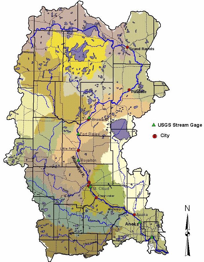
Study Area
Five separate reaches of the Mississippi River above Minneapolis were identified for this project. The upstream most location at Grand Rapids is the controlled outflow from the Pokegama Lake Reservoir. The downstream terminus is the Saint Anthony Falls Lock and Dam in Minneapolis. Listed in order from upstream to downstream, they are:
Grand Rapids to Aitkin, MN
Aitkin to Little Falls, MN
Little Falls to St Cloud, MN
St Cloud to Anoka, MN
Anoka to Minneapolis, MN
Study Area Map
Hydrology
The three sets of flow conditions were defined in previous subject studies as:Low Flow: Discharges exceeded 90 percent of the time based on the period of record.
Medium Flow: Discharges exceeded 50 percent of the time based on the period of record.
High Flow: Discharges exceeded 10 percent of the time based on the period of record.
The US Geological Survey publishes daily river discharges for rivers and streams in the United States. Only those daily discharges marked as Approved for Publication by the USGS were used. For the period of record at each USGS gaging station, discharge data values were retrieved and numerically sorted. By inspection, discharges which fell at the 90, 50, and 10-percentile points were then used. Comparison to discharges used in previous studies showed this method to be in agreement. The results of the annual flow duration analysis may be found in the complete report furnished to the sponsor.
Selected Tributaries
The following travel time estimates were prepared for the Upper Mississippi River Source Water Protection Project by the U.S. Geological Survey for the Sauk, Elk, Crow and Rum Rivers and Elm, Coon, and Rice Creeks. Estimates were prepared for High, Medium, and Low Flow conditions (flows exceeded 10%, 50%, and 90% of the time, respectively) from selected points on the tributary to its confluence with the Mississippi River.
| River | Location | High Flows | Medium Flows | Low Flows |
|---|---|---|---|---|
| Sauk River | County Road 1 | 0.03 hr | 0.04 hr | 0.1 hr |
| Veterans Drive | 2.01 hr | 2.51 hr | 6.79 hr | |
| County Road 121 | 5.10 hr | 6.33 hr | 16.84 hr | |
| Interstate 94 Bridge | 5.69 hr | 7.07 hr | 18.75 hr | |
| County Road 139 (Rockville) | 8.56 hr | 10.62 hr | 27.89 hr | |
| Elk River | Orono Lake Dam | 0.61 hr | 1.05 hr | 1.48 hr |
| Orono Lake inlet | 2.25 hr | 3.77 hr | 5.23 hr | |
| BN Railroad | 4.38 hr | 7.35 hr | 10.21 hr | |
| USGS gauge | 5.95 hr | 9.98 hr | 13.84 hr | |
| Crow River | Interstate 94 Bridge | 3.42 hr | 8.39 hr | 15.24 hr |
| St. Michael WWTP | 5.68 hr | 14.20 hr | 26.48 hr | |
| Rockford USGS gauge | 10.9 hr | 27.25 hr | 50.84 hr | |
| Rum River | Below Trott Brook | 5.78 hr | 10.14 hr | 15.44 hr |
| County Road 22 USGS gauge | 9.84 hr | 17.28 hr | 26.41 hr | |
| Elm Creek | US 169 | 0.31 hr | 0.75 hr | 1.18 hr |
| Elm Creek Road USGS gauge | 4.28 hr | 9.60 hr | 14.23 hr | |
| Below Rush Creek confluence | 5.46 hr | 12.24 hr | 18.11 hr | |
| 93rd Ave N | 8.89 hr | 20.09 hr | 29.93 hr | |
| Coon Creek | Northdale Blvd | 4.95 hr | 6.98 hr | 11.58 hr |
| S Coon Creek Drive | 8.82 hr | 12.41 hr | 20.49 hr | |
| Rice Creek | Long Lake Rd | 4.61 hr | 6.39 hr | 11.20 hr |
| Baldwin Lake outlet | 10.43 hr | 14.37 hr | 24.79 hr |
Time of Travel Methodology
Times of travel were computed using the travel time option of the REMM model. Basic hydraulic data for the model consists of a family of stage-discharge-velocity relationships at locations where hydraulic and hydrologic data are available. The data were taken from USGS measurements supplemented with hydraulic data and computations from other engineering studies such as FEMA flood insurance studies.
Repetitive model simulations were run using the discharges for low, medium, and high flow conditions. The time of travel between any two locations within a reach of river was computed by inputting the flow rate in cubic feet per second (CFS), at the upstream and downstream ends of the model. Since the flow rates are all year values; the month, day, and initial time values are independent variables. For this study, July 1st at midnight was used at the upstream location. Using this technique it was possible to produce output in days, hours, and minutes directly without any additional correction.
Chart Development
To populate the travel time values for one travel chart for a given flow condition, it was necessary to execute repetitive simulations of the REMM model. Each model simulation produced the time of travel from one upstream location to all of the downstream landmark locations.
This scenario was repeated beginning at the upstream-most location and progressing downstream one landmark location for the next simulation.
To meet the simulation requirements, minimize errors, and provide a homogeneous computational environment, a series of Linux and Perl language programs was developed to produce one chart for one flow condition with a single execution.
The methodology described above was used for each flow condition within a reach, and then in turn for each of the five river reaches. The times of travel required for one flow condition within a given reach of river may be determined by the sum of powers of integers formulation; where the power is unity.
For example; for a reach of river with 25 landmarks, the total number of times of travel computed would be:
SUM = 25 + 24 + 23 ....... + 3 + 2 +1 = 325
The sum of these values is 325. The number of simulations required for one flow condition is equal to the number of landmarks. Given that 25 landmarks is typical for each reach of river, 75 simulations were conducted for each of the five river reaches, yielding a total of 375 simulations for the study area.
Chart Usage
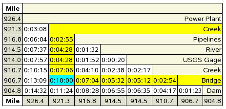
The time of travel charts are modeled in the style of road maps which allow for a quick determination of the travel distance between any two points on the map. The same technique can be applied to times of travel on a river or stream given a flow condition. With a time of travel chart in hand, one can look up the travel time by choosing any two locations and finding their point of commonality.
River mileages are shown along the left and bottom of the charts. Landmarks corresponding to these river mileages are shown from top to bottom along the right hand border of the charts.
In the sample chart below, the time of travel between the site labeled as Creek and that noted as Bridge is shown as approximately 0:10:00 or 0 days, 10 hours, and 00 minutes.
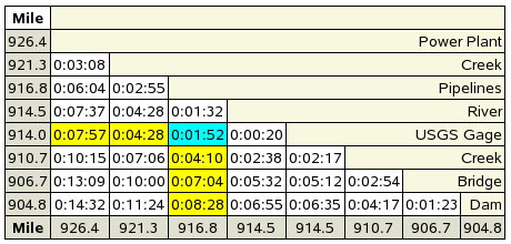
In the next chart shown below, where the river mileages may be more meaningful or common than landmarks, river mileages are shown in lieu of landmark place names.
Given two river mileages, in this case 914.0 along the left vertical edge and 916.8 along the bottom edge of the chart, one can find the river mile for one landmark along the left hand side of the chart and the other along the bottom, then locate the point in common as shown below.
Limitations
Travel times were determined for open water, surface current, all season river discharges. If other physical elements may be important, the following guidelines are offered:
Wind: Times of travel at the surface can be affected by wind action. This is especially true in areas where the river is wide and winds may blow material toward and eventually onto the shore. Winds blowing downstream or upstream may have either a beneficial or adverse impact.
Ice cover: Reduce the time of travel by 10-percent as the bottom of ice friction and resulting velocity profile changes.
Velocities at other depths: If the average velocity in the vertical water column is needed, use 90 to 95-percent of the surface current velocity. Travel times for materials near the bottom of the river is harder to estimate as depth of flow and the roughness of the channel bottom may vary considerably and is difficult to estimate with any degree of certainty.
Seasonal variability: Flows are generally low during the winter season after an ice cover is formed. During the spring snow melt runoff in late March and early April, flow rates are generally higher. Summer rainfalls may produce noticeable increases in flow rates following storms. During the fall and early winter, flows are usually lower than normal.
Dams and Control Structures: Hydraulic control structures such as dams, navigation locks, and hydropower facilities create pools of slack water upstream. In these pools, flow velocities are typically much slower than those upstream in run of the river reaches. Dams of significant height typically create pools of significant length. Immediately downstream, local flow velocities are significantly higher than run of the river and the river is more turbulent. During periods of drought, such in 1988, these pools can account for significant evaporation. As a result the records may show lower flow rates in these areas compared to upstream and downstream.
Summary
The cities of St. Cloud, Minneapolis, and St. Paul obtain most of their drinking water from the Mississippi River. Emergency responders and water managers need a reliable estimate of travel times for low, medium, and high flow conditions in a simple, easy to use format in hard copy form. Hard copy Times of Travel Charts in a format similar to road map mileage charts provide this information which can be used in settings ranging from an office to an individual in the field without a computer or other automation tools.
Selected References
U.S. Army Corps of Engineers, 1997, Mississippi River Defense Network Spill Response Manual: U.S. Army Corps of Engineers, St Paul District.
Pomerleau, Richard, P.E., August 1997, Riverine Emergency Management Model: U.S. Army Corps of Engineers, St Paul District.
Arntson, A.D., Lorenz, D.L., and Stark, J.R., 2004 Estimation of travel times for seven tributaries of the Mississippi River, St. Cloud to Minneapolis, Minnesota, 2003: U.S. Geological Survey Scientific Investigation Report 2004-5192, 17p.
Additional Formats
This report is also available in PDF